Mouse embryo GEO-seq data

Here we use a small GEO-seq dataset to demonstrate the simple usage of STRIDE. The GEO-seq data was derived from the study of early mouse embryo (Peng et al., Nature, 2019), and the scRNA-seq data was collected from another multi-omics study (Argelaguet et al., Nature, 2019). Only data of E7.5 are used in this example. Users can download the demo data from here.

Step 1 Deconvolve the cell-type composition of GEO-seq data

The first step of STRIDE is to infer the cell-type-associated topic profiles from scRNA-seq. Next, the pre-trained topic model could be employed to infer the topic distributions of each spot in spatial transcriptomics. Finally, STRIDE could estimate the cell-type fractions of each spot by combining cell-type-by-topic distribution and topic-by-spot distribution. All these steps are implemented by STRIDE deconvolve function.

STRIDE deconvolve --sc-count Data/scRNA_E7.5_gene_count.txt \
--sc-celltype Data/scRNA_E7.5_lineage.txt \
--st-count Data/GEO-seq_E7.5_gene_count.txt \
--outdir Result/STRIDE --outprefix GEO-seq_E7.5 --normalize

The results of STRIDE deconvolve will be stored in the Result/STRIDE floder, and the detailed descritions are shown as below.

File	Description
model/	The directory stores topic models trained using the scRNA-seq data.
Model_accuracy_plot.pdf	The accuracy of cell-type assignment of single cells in scRNA-seq data, which is used to select the optimal topic number.
Prediction_truth_heatmap_BayesNorm_{topicnum}.pdf	The confusion matrix for the selected topic model, which reflects the consistency between the prediction and the truth for the scRNA-seq data.
{outprefix}_spot_celltype_frac.txt	The deconvolved cell-type fractions for all spots.
{outprefix}_topic_spot_mat_{topicnum}.txt	The topic distribution for all spots. The ‘topicmun’ is the optimal topic number automatically selected by STRIDE.

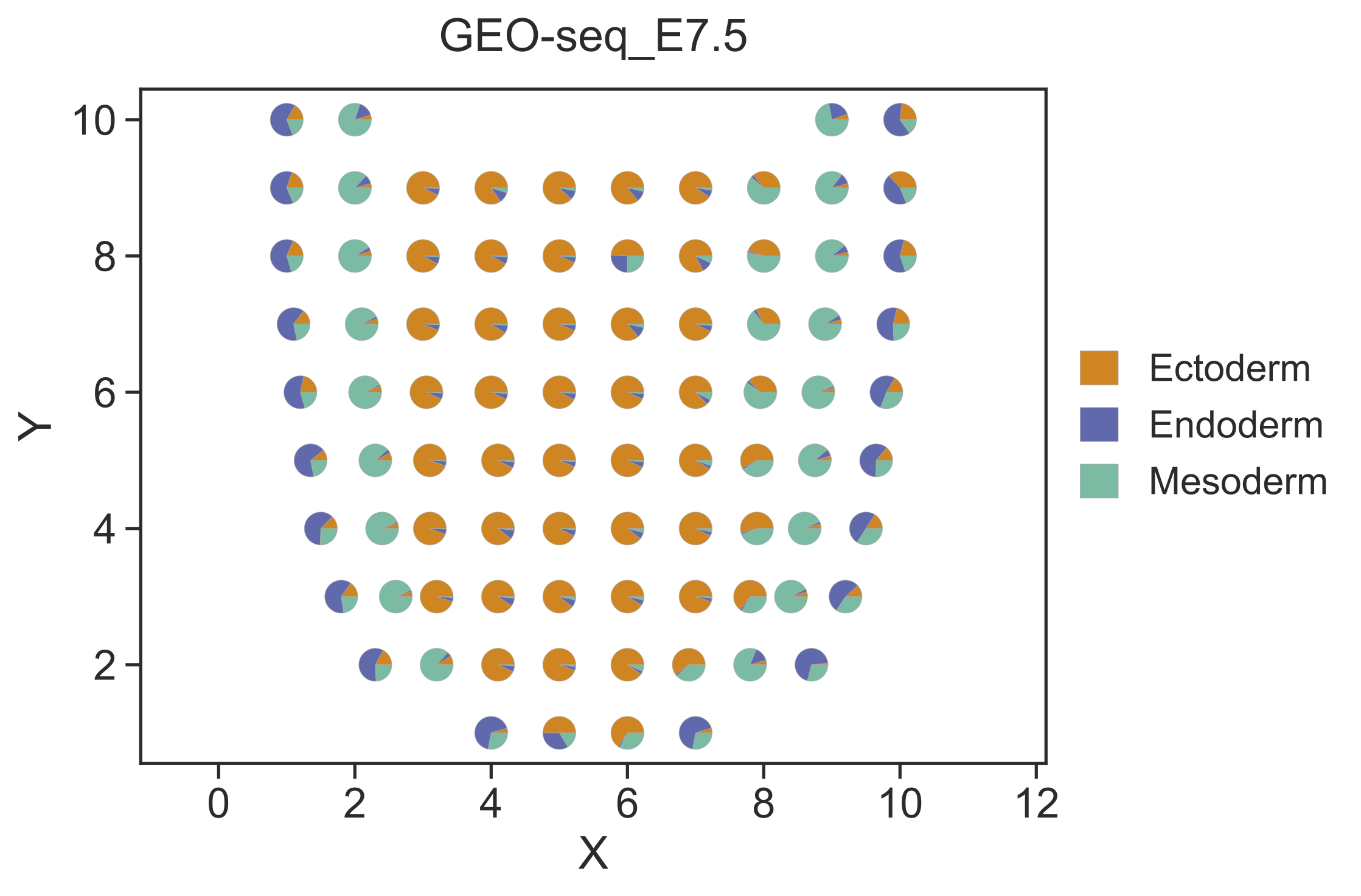
Step 2 Visualize the deconvolution result

After cell type deconvolution, STRIDE plot could be used to visualize the deconvolution result. Users can choose either the scatterpie plot or the scatter plot by setting --plot-type.

STRIDE plot --deconv-file Result/STRIDE/GEO-seq_E7.5_spot_celltype_frac.txt \
--st-loc Data/GEO-seq_E7.5_location.txt --plot-type scatterpie --pt-size 13 \
--outdir Result/STRIDE --outprefix GEO-seq_E7.5

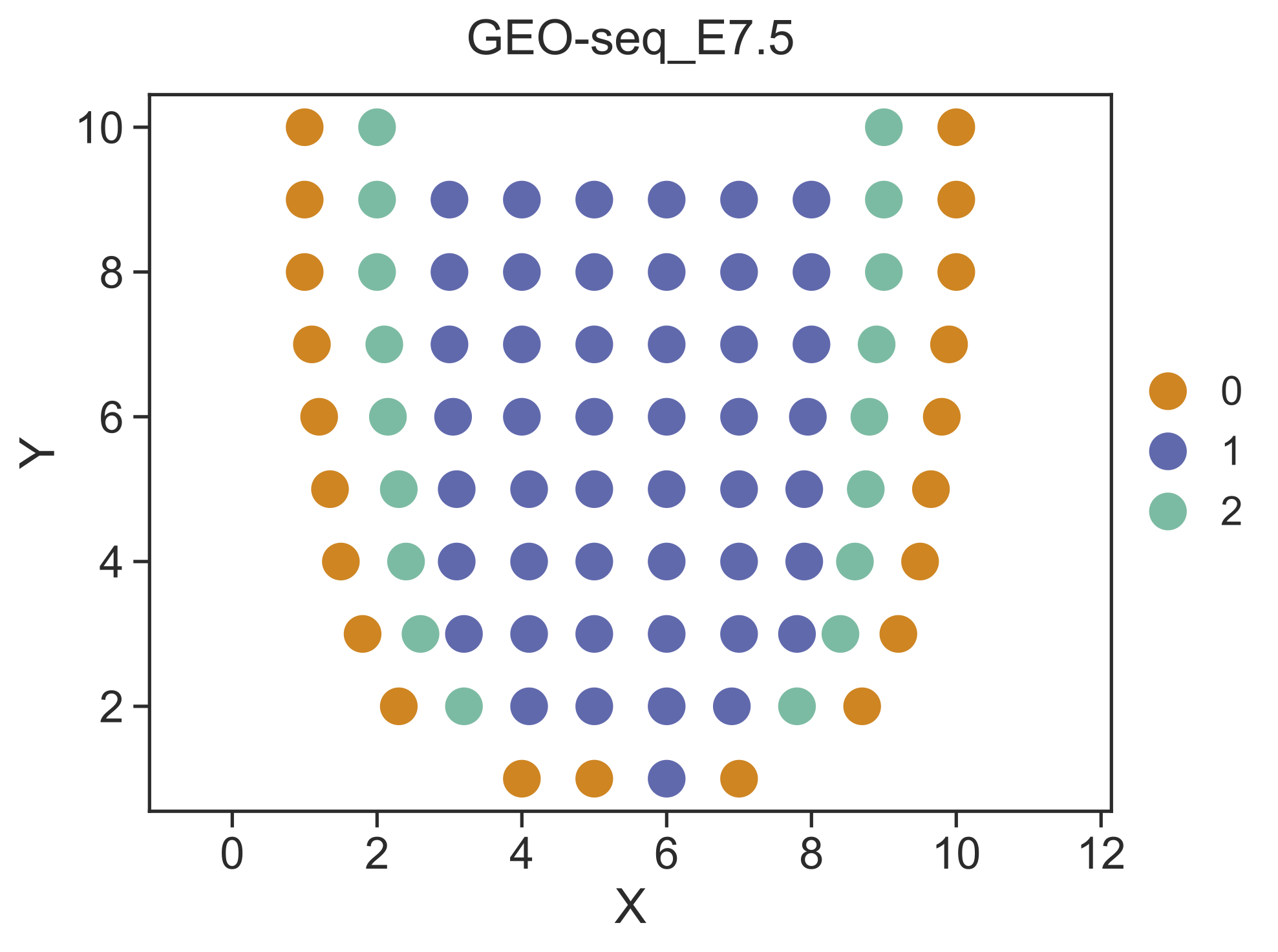
Step 3 Identify spatial domains

STRIDE could further identify the spatial domains by combining both the neighborhood information and the cell-type deconvolution result. Locations with similar cell-type compositions and similar surrounding cell populations will be clustered together.

STRIDE cluster --deconv-file Result/STRIDE/GEO-seq_E7.5_spot_celltype_frac.txt \
--st-loc Data/GEO-seq_E7.5_location.txt --plot --pt-size 13 \
--weight 0.5 --ncluster 3 \
--outdir Result/STRIDE --outprefix GEO-seq_E7.5